
An end-to-end, reproducible Λ⁰ analysis
Last updated on 2026-09-30 | Edit this page
Estimated time: 55 minutes
Overview
Questions
- How do assistant + server + skill compose into one analysis?
- How does the kernel scale from one file to the full sample?
- How is the yield extracted and made reproducible?
Objectives
- Set up any MCP client for the end-to-end run in three steps.
- Scale the analysis from one file to a full dataset.
- Accept or reject an agent-produced yield using the audit checklist.
Run it in your client
In eic-shell, in your analysis directory:
BASH
eic-mcp up
eic-mcp config opencode
R=https://raw.githubusercontent.com/eic/tutorial-mcp/main/files/skills
curl -fsSLO $R/AGENTS.md
curl -fsSL --create-dirs -o .opencode/skills/lambda-fit/SKILL.md $R/lambda-fit/SKILL.md
opencode
Check that /mcp lists uproot,
xrootd, and rucio, then paste the prompts
below. For Claude Code, use eic-mcp config claude and
.claude/skills/.
The composed pipeline
The skill (Episode 4) gives the steps, the uproot server (Episode 3) reads the data, and the agent loop (Episode 1) runs and checks it.
%%{init: {'theme':'base', 'themeVariables': {'fontSize':'15px','lineColor':'#94a3b8','edgeLabelBackground':'#e2e8f0','clusterBkg':'#1f293720','clusterBorder':'#94a3b8','titleColor':'#94a3b8'}}}%%
flowchart LR
    accTitle: {End-to-end agent run}
    accDescr: {End-to-end agent run}
    A["resolve input<br/>root:// file or file list"]:::data --> B["build m(p,π) histogram<br/>uproot MCP"]:::tool
    B --> C["fit Gaussian + poly-2<br/>opencode prompt"]:::tool
    C --> D["report μ, σ, S, χ²/ndf<br/>+ plot + provenance"]:::out
    classDef data fill:#fff4e0,stroke:#f08c00,stroke-width:1.5px,color:#5c3b00;
    classDef tool fill:#e6f7ed,stroke:#2f9e44,stroke-width:1.5px,color:#0b3d1f;
    classDef out fill:#f3e8ff,stroke:#7048e8,stroke-width:1.5px,color:#2e1065;
One file, end to end
With the three servers running and the lambda-fit skill available,
one request runs the whole chain. Point it at one of the dataset’s
root:// files. The assistant uses rucio tools
to find a DIS dataset and list_file_replicas for the URLs,
xrootd to confirm the file is there, then reads it in
place:
Using the lambda-fit skill, measure the Lambda0 peak in this file:
root://epicxrd1.sdcc.bnl.gov:1095//... (one root:// file of the campaign 26.04.1
BeAGLE eCu ep 10x115 dataset from Episode 3's exercise).
Build the proton-pion invariant-mass histogram with the uproot MCP server (tree 'events'),
fit it, and report mu, sigma, the yield, and chi2/ndf, with the plot, or report insufficient
statistics if the fit window is too sparse.
The assistant builds the histogram with the uproot server, then fits it. If your model stops after the histogram (small models do), paste the fit as its own request:
Fit the histogram you just built with execute_kernel: a Gaussian plus a 2nd-order polynomial
over [1.08, 1.16] GeV. Report mu, sigma, the signal yield S, and chi2/ndf, checked against
the lambda-fit skill's success criteria.
One file gives only ~8 candidates in the fit window, so the correct answer is insufficient statistics: the skill says to stop instead of fitting, and a model that quotes \(\mu\) anyway has ignored it. The peak at \(\mu \approx 1.1157\) GeV comes from the larger sample below.
Smaller models take shortcuts: check the result, not the route
A smaller model may call different tools than the skill says and still get the same histogram. The audit checklist below judges the result, not the route.
Scaling to the full sample
The same calculation can run over many files and return one merged histogram:
Using the lambda-fit skill, run the same proton-pion mass kernel across the first 8 files of the
campaign 26.04.1 BeAGLE eCu ep 10x115 dataset with execute_kernel_dataset (tree 'events'),
merge the histograms, then fit the result and report mu, sigma, the yield, and chi2/ndf
for both Lambda and anti-Lambda, with the plot.
Eight files take about a minute (paste the fit prompt above if it stops). For more files, run background jobs in batches of ~20 files and let the assistant wait for them:
Using the lambda-fit skill, run the proton-pion mass kernel over the first 100 files of the
campaign 26.04.1 BeAGLE eCu ep 10x115 dataset. Submit it with submit_kernel_dataset
(tree 'events') in batches of about 20 files, poll get_job_status until every job finishes,
fetch the histograms with get_job_result and merge them, then fit and report mu, sigma,
the yield, and chi2/ndf for both Lambda and anti-Lambda, with the plot.
Over ~100 files this gives the reference spectrum below: a clear Λ⁰ (and Λ̄) peak over the combinatorial background.
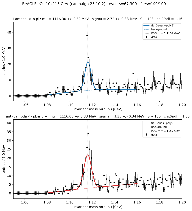
OUTPUT
Lambda      -> p pi-:   mu = 1116.30 +/- 0.32 MeV   sigma = 2.72 +/- 0.33 MeV   S = 123   chi2/ndf = 1.16
anti-Lambda -> pbar pi+: mu = 1116.06 +/- 0.33 MeV   sigma = 3.35 +/- 0.34 MeV   S = 160   chi2/ndf = 1.05
The fitted \(\mu\) sits ~0.6 MeV above the PDG value (1.115683 GeV), a calibration-level offset typical of reconstructed momenta; \(\sigma\) is the detector mass resolution, not the (negligible) Λ⁰ natural width.
Extracting the yield
The fit model is a Gaussian signal on a second-order polynomial background over \([1.08, 1.16]\) GeV:
\[ f(m) = A \exp\!\left[ -\tfrac{1}{2} (m - \mu)^2 / \sigma^2 \right] + \left( c_0 + c_1 (m - m_\Lambda) + c_2 (m - m_\Lambda)^2 \right) \]
The polynomial absorbs the combinatorial background (Episode 2); the integrated signal is \(S = A\sqrt{2\pi}\,\sigma / (\text{bin width})\). Report \(S\) with its uncertainty alongside \(\mu\), \(\sigma\), and \(\chi^2/\text{ndf}\); a bare bin count mixes signal with background.
Audit
Audit checklist
- Signal. \(\mu\) within a few MeV of 1.115683 GeV; \(\sigma\) consistent with detector resolution; \(\chi^2/\text{ndf}\) of order unity; \(S\) reported with an uncertainty.
- Inputs pinned. Dataset (campaign and file list), particle masses, mass window, binning, and fit range all fixed and recorded.
- Provenance. Tool calls and their arguments logged, so the run can be reconstructed.
- Cost bounded. A few files during development before scaling up.
- Oversight. A human inspected the fit before the result was reported.
Exercises (specification)
- Run the single-file chain through your assistant and report \(\mu\), \(\sigma\), \(S\), and \(\chi^2/\text{ndf}\).
- Process 8 files and compare the fit to the ~100-file result; comment on the statistical uncertainty.
- Complete the audit checklist for your run, attaching the recorded tool calls as provenance.
Try a different beam
The same prompt works with any reconstructed-DIS DID. Nuclear beams (eCu, eAu) give the most Λ per event; ep samples need a few times more files.
The final episode lists the other MCP servers the EIC provides.
- One prompt runs the whole Λ⁰ analysis, from one file up to the full dataset.
- Check the fit against the audit checklist before you trust it.