
All in One View
Content from Introduction
Last updated on 2026-07-11 | Edit this page
Overview
Questions
- Why should I be interested in track-cluster matching?
Objectives
- Understand physical motivation behind examples in tutorial
Like we noted in the Setup section, our goal in this tutorial is to understand how to use the PODIO interface in an analysis. As such, this tutorial will build on the earlier Analysis Tutorial, which discussed how to analyze our reconstruction output with the ROOT TTreeReader and RDataFrame.
Our vehicle for doing so will be two commmon and complementary analysis routines:
- Matching tracks and clusters; and
- Matching truth objects to their reconstructed counterparts.
On one hand, the former utilizes purely reconstructed objects (tracks and clusters) and will illustrate the basics of PODIO. While on the other hand, the latter utilizes purely simulated objects (generated particles) and will illustrate how to navigate relations and associations.
We’ll deploy these routines to study \(J/\psi\) decaying to \(e^{+} + e^{-}\) pairs, a common decay channel used in many areas of EIC science.
Why these?
Before diving into PODIO, though, I would like to motivate why you should care about these two routines. To start, remember that a particle is not just a track, a cluster, or so on. A particle will leave signals in several detectors. The majority of particles in a typical DIS event will create hits in our trackers and will shower — forming a cluster — in at least one of our calorimeters.
This is illustrated in the following image, where the colored bands indicate the tracking layers (orange), cherenkov detector (pink), electromagnetic calorimeter (ECal, purple), magnet solenoid (grey), and hadronic calorimeter (HCal, blue) in ePIC’s barrel.
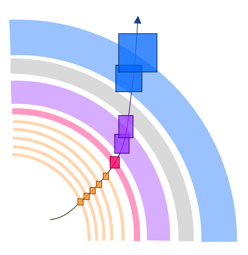
Accurately reconstructing the particle — its momentum, energy, charge, mass — will require us to make use of all of this information. For example, an electron will create a track and will usually deposit all of its energy into an ECal. In contrast, a charged hadron like a \(\pi^{-}\)), will frequently deposit energy into HCal, while a \(\pi^{0}\) will deposit energy into an ECal without creating a track. This is illustrated in the following figure.
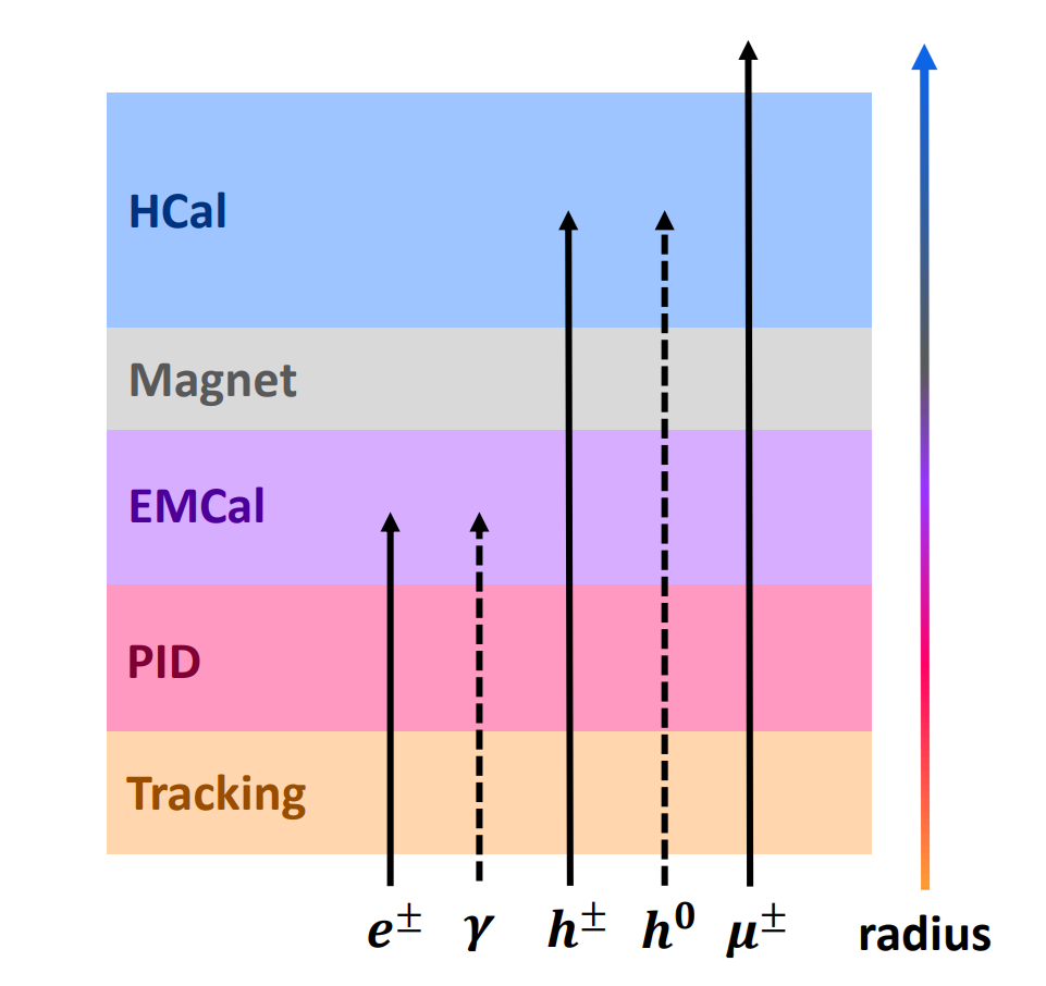
Therefore, track-cluster matching is a critical step in our reconstruction, which we use to identify leptons, measure neutral particles, and more. In this tutorial, we’ll use it identify decay \(e^{\pm}\) which we’ll reconstruct a \(J/\psi\) from.
To validate our reconstructed \(J/\psi\), however, we’ll need to identify the corresponding simulated particles and compare them. That’s where the truth-reco matching comes in.
References
- Track-cluster is a critical part of reconstructing particles
- Truth-reconstructed matching is needed to validate reconstructed particles
Content from Using PODIO to Work With Our Data Model
Last updated on 2026-07-11 | Edit this page
Overview
Questions
- What is our data model?
- What is PODIO?
- How do I interface with our data model?
Objectives
- Understand relationship between the data model and PODIO
- Become familiar with PODIO concepts and synatx
The EDM4eic Data Model
A data model is how we represent our data in our software. In other words, a standardized set of data structures that we use to pass information between different parts of our software stack (DD4hep, EICrecon, etc.) and between different algorithms in those parts.
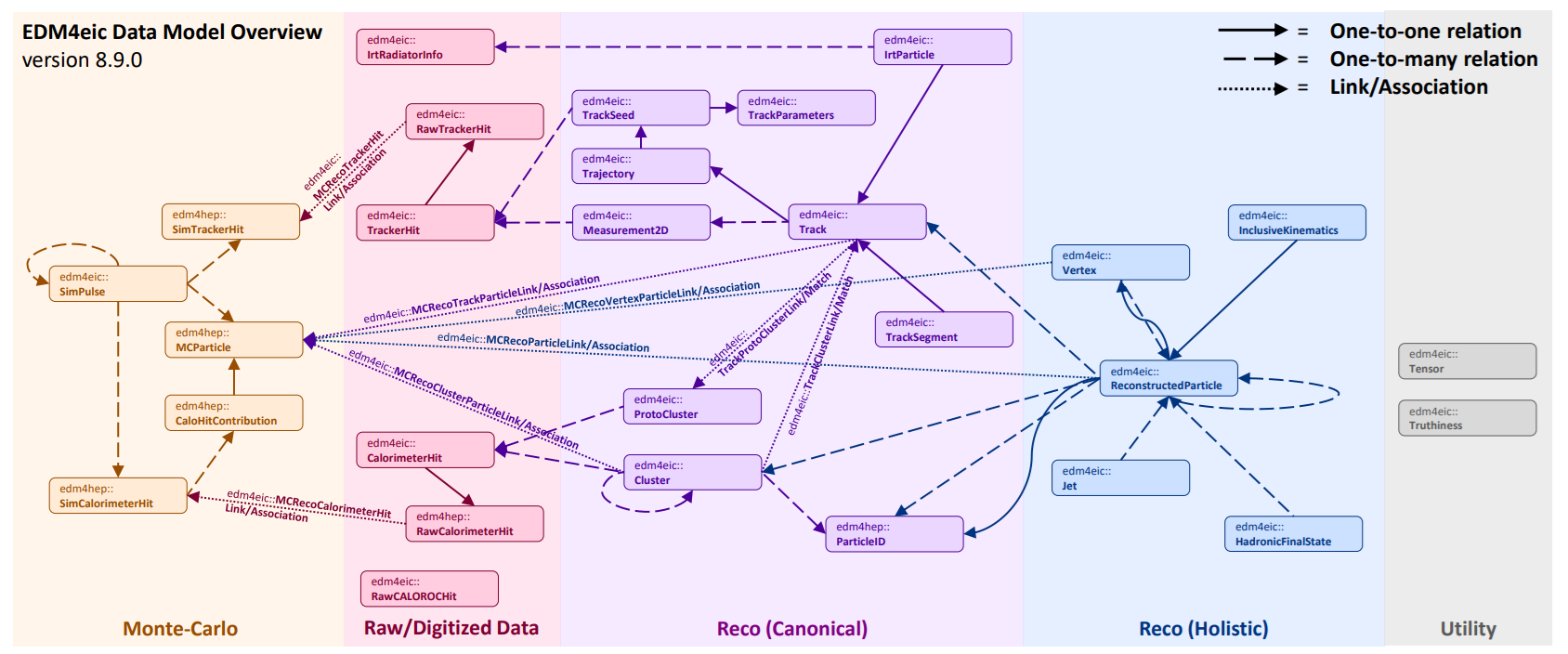
Our data model is EDM4eic (Event Data Model for EIC), and is summarized in the above figure. Each box corresponds to a data structure, and the arrows correspond to connections between these structures. The entire model is defined in a single YAML file, edm4eic.yaml, which we’ll break down in detail below.
Exercise
Take a moment to scan the figure, paying attention to the names of
structures. Then pick a structure and find it in the YAML file mentioned
above: notice how the arrows correspond to the fields labeled
OneToOneRelations or OneToManyRelations.
For example, edm4eic::Cluster has one-to-many relations
to edm4eic::CalorimeterHit (the hits combined to form the
cluster), to other edm4eic::Clusters, and to
edm4hep::ParticleID. Each of these corresponds to an arrow
leaving the cluster box in the figure.
A few things comments before we move on:
- Using a standardized set of structures helps keep our software modular, meaning we can easily swap out parts, since all our data adheres to standardized interfaces;
- The data model does not say anything about input/output formats: we write our data using ROOT, but we could also write it in other formats like HDF5;
- And we want our model to be predictable and intuitive: accessing the energy of a calorimeter cluster should be identical to accessing the energy of a particle.
Note
We also utilize the EDM4hep data model in our software. This is a data model developed by the Key4hep project, which is developing common software to support the FCC, ILC/CLIC, Muon Collider, and more. Just like with our data model, the EDM4hep model is also defined in a single YAML file, edm4hep.yaml.
An Introduction to PODIO
So then what’s PODIO? PODIO (Plain-Old-Data Input/Output) is a toolkit for generating and managing a data model like EDM4eic. It reads in a YAML file like edm4eic.yaml and generates all the C++ and Python code needed to read, write, and interface with the structures defined in there.
Classes
Let’s look at one of these structures:
YAML
edm4eic::Track:
  Description: "Track information at the vertex"
  Author: "S. Joosten, J. Osborn"
  Members:
    - int32_t           type                       // Flag that defines the type of track
    - edm4hep::Vector3f position                   // Track 3-position at the vertex
    - edm4hep::Vector3f momentum                   // Track 3-momentum at the vertex [GeV]
    - edm4eic::Cov6f    positionMomentumCovariance // Covariance matrix in basis [x,y,z,px,py,pz]
    - float             time                       // Track time at the vertex [ns]
    - float             timeError                  // Error on the track vertex time
    - float             charge                     // Particle charge
    - float             chi2                       // Total chi2
    - uint32_t          ndf                        // Number of degrees of freedom
    - int32_t           pdg                        // PDG particle ID hypothesis
  OneToOneRelations:
    - edm4eic::Trajectory trajectory // Trajectory of this track
  OneToManyRelations:
    - edm4eic::Measurement2D measurements // Measurements that were used for this track
    - edm4eic::Track         tracks       // Tracks (segments) that have been
                                          // combined to create this track
This is an example of a class. At the top of the definition,
we see some basic info like the name of the structure, a brief
description, and the authors. Following this, we see a block labeled
Members. These are your basic class members. Suppose we
have an edm4eic::Track named track, how would
we access its members?
PYTHON
# getting data members
trk_time = track.getTime()
trk_ndf  = track.getNdf()

# setting data members
track.setCharge(-1.0)
track.setPDG(11)
Or in C++:
CPP
// getting data members
float    trk_time = track.getTime();
uint32_t trk_ndf  = track.getNdf();

// setting data members
track.setCharge(-1.0);
track.setPDG(11);
This already highlights of the big advantages of using PODIO to work with our data: the interface is almost identical between C++ and Python. We’ll see where they diverge in later sections.
Wait! But how would I know that the accessors start with
get or set? 1. First, look at the top of the
YAML file: you’ll notice under options that getSyntax is
set to true. This means that the accessor functions for
class members will always start with
get/set, letting you infer what the
relevant functions are from the YAML. 2. You can also look at the
generated classes on our EDM4eic doxygen page. Or while
you’re in eic-shell, you can look at them in the path
/opt/local/include/edm4eic.
Exercise
Follow the link to the
doxygen page, and locate the header file for
edm4eic::Track. Once you found it, give it a quick scan.
Then in eic-shell, find the same header file and compare it to the
online version.
On the doxygen page, the header is listed under
edm4eic/Track.h. In eic-shell, the same file is at
/opt/local/include/edm4eic/Track.h — you can view it with,
e.g., less /opt/local/include/edm4eic/Track.h. You’ll find
the same getTime(), getNdf(), etc. accessors
that the YAML file implies.
Collections and Frames
For reading in/writing out classes, they’ll need to be placed in a
collection. Collections can be thought of as almost (but not
quite!) a c++ std::vector or Python list of objects.
Iterating through their contents looks like you’d expect for either of
those containers:
PYTHON
tracks = frame.get("CentralCKFTracks")
for track in tracks:
    chi2_ndf = track.getChi2() / track.getNdf()
Or:
CPP
auto& tracks = frame.get<edm4eic::TrackCollection>("CentralCKFTracks");
for (const auto& track : tracks) {
  chi2_ndf = track.getChi2() / track.getNdf();
}
The frame in the above snippets is a Frame,
which holds and organizes several collections. We’ll see frames and
collections in action in the following episodes. However, a detailed
explanation of their usage is outside the scope of this tutorial.
Warning
The big thing to note here is that collections are read-only! This means that you can’t modify an object you are reading from a collection!
Components
Notice that the position and momentum of the track are stored as an
edm4hep::Vector3f. This is an example of a
component. Let’s look at the definition:
YAML
edm4hep::Vector3f:
  Members:
    - float x
    - float y
    - float z
  ExtraCode:
    includes: "#include <cstddef>"
    declaration: |
      constexpr Vector3f() : x(0),y(0),z(0) {}
      constexpr Vector3f(float xx, float yy, float zz) : x(xx),y(yy),z(zz) {}
      constexpr Vector3f(const float* v) : x(v[0]),y(v[1]),z(v[2]) {}
      constexpr bool operator==(const Vector3f& v) const { return (x==v.x&&y==v.y&&z==v.z) ; }
      constexpr bool operator!=(const Vector3f& v) const { return !(*this == v) ; }
      constexpr float operator[](unsigned i) const {
        static_assert(
          (offsetof(Vector3f,x)+sizeof(Vector3f::x) == offsetof(Vector3f,y)) &&
          (offsetof(Vector3f,y)+sizeof(Vector3f::y) == offsetof(Vector3f,z)),
          "operator[] requires no padding");
        return *( &x + i ) ;
      }
It has 3 data members and some extra code, which just defines some
handy functions. If you find this in edm4hep.yaml,
then you’ll notice it’s defined under a block labeled
components. Notice that edm4eic::Track is
defined under a block labeled classes.
Components are just simple structs (in the C++ sense).
This means that component accessors are not prefixed by
get/set. For example:
Or:
CPP
#include <cmath>
float px = track.getMomentum().x;
float py = track.getMomentum().y;
float pt = std::hypot(px, py);
Also note that components can’t be stored in a collection and so
can’t be written out except as part of a class such as
edm4eic::Track.
Vector Members
Let’s look at the definition of a calorimeter cluster:
YAML
edm4eic::Cluster:
  Description: "EIC hit cluster, reworked to more closely resemble EDM4hep"
  Author: "W. Armstrong, S. Joosten, C.Peng"
  Members:
    - int32_t              type                         // Flag-word that defines the
                                                        // type of the cluster
    - float                energy                       // Reconstructed energy of the
                                                        // cluster [GeV].
    - float                energyError                  // Error on the cluster energy [GeV]
    - float                time                         // [ns]
    - float                timeError                    // Error on the cluster time
    - uint32_t             nhits                        // Number of hits in the cluster.
    - edm4hep::Vector3f    position                     // Global position of the cluster [mm].
    - edm4eic::Cov3f       positionError                // Covariance matrix of the
                                                        // position (6 Parameters).
    - float                radius                       // Cluster radius [mm].
    - float                dispersion                   // Cluster dispersion [mm].
    - std::array<float, 3> principalAxesLengthsXYZ      // Lengths along the cluster's principal
                                                        // axes [mm], sorted in descending order
                                                        // (equivalent to sqrt of eigenvalues of the
                                                        // position covariance). For an XY planar
                                                        // detector one can expect this to be
                                                        // [sigma_max, sigma_min, 0].
    - std::array<float, 2> principalAxesLengthsThetaPhi // Lengths along the cluster's principal
                                                        // axes [rad], sorted in descending order.
    - float                intrinsicTheta               // Intrinsic cluster propagation direction
                                                        // polar angle [rad].
    - float                intrinsicPhi                 // Intrinsic cluster propagation direction
                                                        // azimuthal angle [rad]. For an XY planar
                                                        // detector one can expect this to be the
                                                        // tilt of "sigma_max" axis.
    - edm4eic::Cov2f        intrinsicDirectionError     // Error on the intrinsic cluster
                                                        // propagation direction
  VectorMembers:
    - float shapeParameters     // [DEPRECATED] use radius, dispersion,
                                // principalAxesLengthsXYZ/ThetaPhi instead.
    - float hitContributions    // Energy contributions of the hits. Runs parallel to ::hits()
    - float subdetectorEnergies // Energies observed in each subdetector used for this cluster.
  OneToManyRelations:
    - edm4eic::Cluster        clusters    // Clusters that have been combined to form this cluster
    - edm4eic::CalorimeterHit hits        // Hits that have been combined to form this cluster
    - edm4hep::ParticleID     particleIDs // Particle IDs sorted by likelihood
You’ll see a block labeled VectorMembers. These are just
std::vectors of data. For example,
hitContributions holds the weighted energy of the
calorimeter cells (a.k.a hits) that make up a given
cluster.
The accessors are the same as for normal members, except they’ll
return a std::vector (C++) or List (Python).
Suppose we have an edm4eic::Cluster named
cluster:
PYTHON
total_energy = 0.0
for weighted_energy in cluster.getHitContributions():
    total_energy += weighted_energy
Or:
Relations
Now, let’s consider the OneToOneRelations and
OneToManyRelations blocks. These are examples of
relations, references to objects in other collections. We use
these to define a direct, necessary relationship between an
object and one other object (one-to-one) or many other objects
(one-to-many).
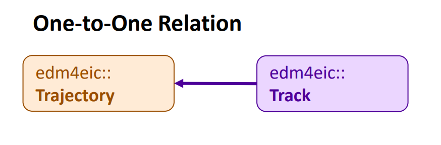
The above figure schematically illustrates a one-to-one relation. A
track should correspond to a charged particle with a defined
momentum and charge. It’s computed from a trajectory, a path
fit to a set of points from our trackers. This relationship is expressed
in the one-to-one relation from our edm4eic::Track to an
edm4eic::Trajectory.
Retrieving the object from a relation is done the same way you would get a value from a member:
Or:
C++
auto     trajectory    = track.getTrajectory();
uint32_t n_points_used = trajectory.getNMeasurements();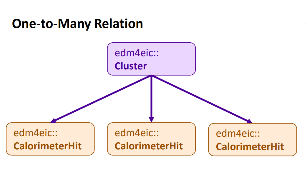
Then the above figure schematically illustrates a one-to-many
relation. For example, a calorimeter cluster is group of calorimeter
cells (hits). The cells that make up a given cluster are recorded in its
one-to-many relation to edm4eic::CalorimeterHits.
Objects referred to in a one-to-many relation are retrieved like you’d expect:
Or:
When you call getHits() in the above snippets, it
returns a List (Python) or std::vector (C++)
of edm4eic::CalorimeterHits just like with vector
members.
Associations/Links
In contrast to relations, which express a direct connection between two or more objects, associations express an indirect connection which might or might not exist. For example, the connection between a monte carlo particle and its reconstructed counterpart:
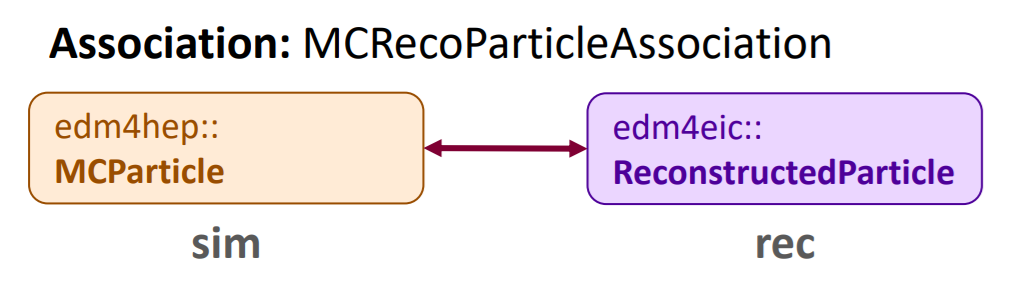
This is defined in edm4eic.yaml as:
YAML
edm4eic::MCRecoParticleAssociation:
  Description: "Used to keep track of the correspondence between MC and reconstructed particles"
  Author: "S. Joosten"
  Members:
    - float weight // weight of this association
  OneToOneRelations:
    - edm4eic::ReconstructedParticle rec  // reference to the reconstructed particle
    - edm4hep::MCParticle            sim  // reference to the Monte-Carlo particle
  ExtraCode:
    includes: "
    #include <edm4eic/ReconstructedParticle.h>\n
    #include <edm4hep/MCParticle.h>\n
    "
    declaration: "
    [[deprecated(\"use getSim().getObjectID().index instead\")]]
    int getSimID() const { return getSim().getObjectID().index; }\n
    [[deprecated(\"use getRec().getObjectID().index instead\")]]
    int getRecID() const { return getRec().getObjectID().index; }\n
      "
The weight here is nominally a measure of the goodness
of the correspondence between the reconstructed and MC particles, and
the rec and sim fields store the references to
the corresponding particles. Let’s assume we have an
edm4eic::MCRecoParticleAssociation called
assoc. Accessing its members is exactly like you’d
expect:
PYTHON
rec_par = assoc.getRec()
sim_par = assoc.getSim()
weight  = assoc.getWeight()
e_frac  = (sim_par.getEnergy() - rec_par.getEnergy()) / sim_par.getEnergy()
Or:
CPP
auto  rec_par = assoc.getRec();
auto  sim_par = assoc.getSim();
float weight  = assoc.getWeight();
float e_frac  = (sim_par.getEnergy() - rec_par.getEnergy()) / sim_par.getEnergy();
Now let’s consider the equivalent link:
YAML
edm4eic::MCRecoParticleLink:
  Description: "Used to keep track of the correspondence between MC and reconstructed particles"
  Author: "S. Joosten"
  From: edm4eic::ReconstructedParticle
  To: edm4hep::MCParticle
There’s a lot less! Links are defined in their own specific
block (labeled links), and only need you to specify which
types they’re connecting (edm4eic::ReconstructedParticle
and edm4hep::MCParticle in this case).
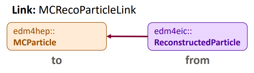
They provide the same functionality as association, but there are a few key differences:
- Links always have the same fields:
from,to, andweight(which is implied); - And they have directionality (illustrated in the above figure).
Point 1 means the accessors will always be the same for any link. The link equivalents of the above snippets are:
PYTHON
rec_par = link.getFrom()
sim_par = link.getTo()
weight  = link.getWeight()
e_frac  = (sim_par.getEnergy() - rec_par.getEnergy()) / sim_par.getEnergy()
And:
CPP
auto  rec_par = link.getFrom();
auto  sim_par = link.getTo();
float weight  = link.getWeight();
float e_frac  = (sim_par.getEnergy() - rec_par.getEnergy()) / sim_par.getEnergy();
The directionality comes into play with the
podio::LinkNavigator, which enables extremely fast lookup
of linked objects. This is, however, outside the scope of this
tutorial.
Warning
We’re in the process of deprecating of associations in favor of links (EDM4hep has already done this). Currently we write out both associations and their equivalent links where needed to not break analysis code. However, we will in the near future remove associations and write out only links
User vs. Storage Layer
Lastly, try opening the file we downloaded during Setup with a ROOT TBrowser:
BASH
$ root --web-display=off lAger3.6.1-1.0_jpsi_10x130_hiAcc_run1.0009.eicrecon.edm4eic.root
root [0] new TBrowser()
Open the tree labeled events and you’ll see hundreds of
branches! Find the branch labeled CentralCKFTracks, open it
and click on a few leaves. This is how PODIO data is organized in
memory, as a big array of structs holding the values in the leaves. This
is referred to as the POD (or Data) Layer.
As noted in the last section, the Analysis Tutorial
illustrates how to work directly with the POD Layer using a ROOT
TTreeReader. The syntax illustrated above is working with
what’s called the User Layer, a think layer of interfaces to
make working with the data easy. A third layer, the Object
Layer, interfaces between the POD and User Layers.
There are clear benefits to working with the User Layer over the POD Layer:
- Significantly less boilerplate code to write,
- Easy, intuitive syntax to deal with relations, associations, and vector members; and
- The User Layer synatx will remain constant, but how the POD Layer is organized may not.
The first two points will be illustrated very clearly in the following episodes. However, there may be cases where working directly with the POD Layer is actually preferable. For example:
- You may want to histogram just one or two members directly, or
- You’re working with a ML pipeline where you’ll need to load the data as a dataframe.
Which analysis method is ultimately up to you: our goal is to support as many methods as possible, and, between the POD Layer and the User Layer, PODIO gives us the tools to do that.
References
- EDM4eic
- EDM4eic YAML File
- EDM4hep
- Key4hep Project
- EDM4hep YAML File
- PODIO
- EDM4eic Doxygen
- PODIO Documentation
- Link Navigator Documentation
- Analysis Tutorial
- A data model is how represent our data in software
- PODIO is a toolkit to generate and interface with data models like EDM4eic
- Classes have their accessors prefixed by get/set, components don’t
- Relations are references to objects in other collections
- Associations/links define indirect connections between objects
Content from Track-Cluster Matching
Last updated on 2026-07-12 | Edit this page
Overview
Questions
- How do actually I use PODIO?
Objectives
- Use PODIO interface to find reconstructed J/psi
Exercise Goal
Now that you have some background, let’s get some hands-on experience with PODIO. Our goal in this epsiode will be to see if we can reconstruct \(J/\psi\) . The next episode will then have us compare these to truth/MC objects.
We’ll build an analysis script/macro up bit-by-bit. But if you’re having trouble placing the code snippets below, you can always refer to the full example scripts for guidance.
Step 0: Skeleton
Overall, our strategy will proceed in two steps:
- Match tracks to ECal clusters and identify electrons with an E/p cut; and then
- Form pairs of electrons and identify J/psi with an invariant mass cut.
The code below will illustrate how to do this using (1) Python and ROOT, and (2) C++ and ROOT (both cases using PODIO). In the future, we’ll expand this tutorial with some extra documents illustrating how to do the same analysis using alternative analysis techniques.
So to begin, let’s 1st create a file. We will suppose the file is
called FindJPsi.py (for the Python version) or
FindJPsi.cxx (for the C++ version), but you are — of course
— free to name the file what you want.
Exercise: Skeleton
Now, in that file, let’s create a skeleton. For Python:
PYTHON
import argparse as ap
import ROOT
import numpy as np

from podio.reading import get_reader

# Default options
in_file_def   = "lAger3.6.1-1.0_jpsi_10x130_hiAcc_run1.0009.eicrecon.edm4eic.root"
out_file_def  = "jpsi_search_py.analysis.root"
match_cut_def = 0.2
ep_min_def    = 0.8
ep_max_def    = 1.2
mass_min_def  = 2.5
mass_max_def  = 3.5

ROOT.TH1.SetDefaultSumw2(True)

def FindJPsi(
    in_file   = in_file_def,
    out_file  = out_file_def,
    match_cut = match_cut_def,
    ep_min    = ep_min_def,
    ep_max    = ep_max_def,
    mass_min  = mass_min_def,
    mass_max  = mass_max_def,
):

    # Open reader and output file ============================================

    # use podio reader to open example EICrecon output
    reader = get_reader(in_file)


    # Event loop ==============================================================

    for frame in reader.get("events"):

        # Grab all the collections we'll need
        particles    = frame.get("MCParticles");
        tracks       = frame.get("CentralCKFTracks");
        clusters_neg = frame.get("EcalEndcapNClusters");
        clusters_cen = frame.get("EcalBarrelClusters");
        clusters_pos = frame.get("EcalEndcapPClusters");
        associations = frame.get("CentralCKFTrackAssociations");


# Main ========================================================================

if __name__ == "__main__":

    # set up argments
    parser = ap.ArgumentParser()
    parser.add_argument("--infile", default = in_file_def)
    parser.add_argument("--outfile", default = out_file_def)
    parser.add_argument("--matchcut", default = match_cut_def)
    parser.add_argument("--epmin", default = ep_min_def)
    parser.add_argument("--epmax", default = ep_max_def)
    parser.add_argument("--massmin", default = mass_min_def)
    parser.add_argument("--massmax", default = mass_max_def)
    args = parser.parse_args()

    # Run calculation
    FindJPsi(
        args.infile,
        args.outfile,
        args.matchcut,
        args.epmin,
        args.epmax,
        args.massmin,
        args.massmax,
    )
And for C++:
CPP
#include <edm4eic/ClusterCollection.h>
#include <edm4eic/MCRecoTrackParticleAssociationCollection.h>
#include <edm4eic/TrackCollection.h>
#include <edm4hep/MCParticleCollection.h>
#include <edm4hep/Vector3f.h>
#include <podio/Frame.h>
#include <podio/ObjectID.h>
#include <podio/ROOTReader.h>
#include <Math/Vector3D.h>
#include <Math/Vector4D.h>
#include <TFile.h>
#include <TH1.h>
#include <cmath>
#include <optional>
#include <map>
#include <memory>
#include <set>
#include <string>
#include <vector>
#include <utility>

TH1::SetDefaultSumw2(kTRUE);

void FindJPsi(
  const std::string& in_file   = "lAger3.6.1-1.0_jpsi_10x130_hiAcc_run1.0009.eicrecon.edm4eic.root",
  const std::string& out_file  = "jpsi_search_cxx.analysis.root",
  const float        match_cut = 0.2,
  const float        ep_min    = 0.8,
  const float        ep_max    = 1.2,
  const float        mass_min  = 2.5,
  const float        mass_max  = 3.5
) {

  // Open reader and output file ==============================================

  podio::ROOTReader reader = podio::ROOTReader();
  reader.openFile(in_file);

  TFile* output = new TFile(out_file.data(), "recreate");

  // Event loop ===============================================================

  while (auto entry = reader.readNextEntry(podio::Category::Event)) {

    auto frame = podio::Frame(std::move(entry));

    // Grab all the collections we'll need
    auto& particles    = frame.get<edm4hep::MCParticleCollection>("MCParticles");
    auto& tracks       = frame.get<edm4eic::TrackCollection>("CentralCKFTracks");
    auto& clusters_neg = frame.get<edm4eic::ClusterCollection>("EcalEndcapNClusters");
    auto& clusters_cen = frame.get<edm4eic::ClusterCollection>("EcalBarrelClusters");
    auto& clusters_pos = frame.get<edm4eic::ClusterCollection>("EcalEndcapPClusters");
    auto& associations = frame.get<edm4eic::MCRecoTrackParticleAssociationCollection>(
      "CentralCKFTrackAssociations");

  }  // end event loop

  // Calculate efficiencies and save output ===================================

  output->cd();
  output->Write();
  output->Close();
  return;

}
Now, just to make sure there are no typos, try running your script with either
for Python. Or:
for C++.
Both commands should finish after a few seconds without printing
anything: the skeleton just reads each event and grabs the collections.
The C++ version will also create an (almost) empty
jpsi_search_cxx.analysis.root. If you see an error about a
missing input file, check that you run the script from the directory
holding the file downloaded during Setup (or point --infile
at it).
During the event loop, notice how we 1st grab a frame
and then grab all of the relevant collections we need from it. Like we
mentioned in the previous episode, a PODIO Frame aggregates
all of the data for all collections in a given category. In this
context, we can think of a single frame as an “event” (a simulated
diffractive event). In our actual data-taking operations, a frame might
be a “timeframe” of streamed data.
A couple notes:
- For thsoe following along in Python who haven’t seen this before,
the chunk at the bottom under
if __name__ == "__main__":is there just make it easy to specify command line arguments. - You might also see how the options in both cases correspond to our 2 steps up above. We’ll see them in action soon.
Next, let’s fill in our histograms. We’ll define all the ones we need for this tutorial. However, we strongly encoourage you to play around and add additional ones!
Exercise: Histograms
Add the following code snippets somewhere near the top of your script/macro. For example right after you open the PODIO reader or right after you create your output file.
PYTHON
    # Create histograms ======================================================

    h_track_momentum_all     = ROOT.TH1D("h_track_momentum_all", "Track #it{p} (all)", 50, 0.0, 10.0)
    h_track_momentum_match   = ROOT.TH1D("h_track_momentum_match", "Track #it{p} (matched to cluster)", 50, 0.0, 10.0)
    h_track_eta_all          = ROOT.TH1D("h_track_eta_all", "Track #eta (all)", 250, -5.0, 5.0)
    h_track_eta_match        = ROOT.TH1D("h_track_eta_match", "Track #eta (matched to cluster)", 250, -5.0, 5.0)
    h_track_cluster_eop      = ROOT.TH1D("h_track_cluster_eop", "Track-cluster E/p", 40, 0.0, 2.0)
    h_invariant_mass         = ROOT.TH1D("h_invariant_mass", "Reconstructed invariant mass", 50, 0.0, 5.0)
    h_daughter_momentum_all  = ROOT.TH1D("h_daughter_momentum_all", "Daughter e^{#pm} #it{p} (all)", 50, 0.0, 10.0)
    h_daughter_momentum_reco = ROOT.TH1D("h_daughter_momentum_reco", "Daughter e^{#pm} #it{p} (reconstructed)", 50, 0.0, 10.0)
    h_daughter_eta_all       = ROOT.TH1D("h_daughter_eta_all", "Daughter e^{#pm} #eta (all)", 250, -5.0, 5.0)
    h_daughter_eta_reco      = ROOT.TH1D("h_daughter_eta_reco", "Daughter e^{#pm} #eta (reconstructed)", 250, -5.0, 5.0)
    h_jpsi_momentum_all      = ROOT.TH1D("h_jpsi_momentum_all", "J/#psi #it{p} (all e^{#pm} decays)", 50, 0.0, 10.0)
    h_jpsi_momentum_reco     = ROOT.TH1D("h_jpsi_momentum_reco", "J/#psi #it{p} (reconstructed e^{#pm} decays)", 50, 0.0, 10.0)
    h_jpsi_eta_all           = ROOT.TH1D("h_jpsi_eta_all", "J/#psi #eta (all e^{#pm} decays)", 250, -5.0, 5.0)
    h_jpsi_eta_reco          = ROOT.TH1D("h_jpsi_eta_reco", "J/#psi #eta (reconstructed e^{#pm} decays)", 250, -5.0, 5.0)
CPP
  // Create histograms ========================================================

  TH1D* h_track_momentum_all     = new TH1D("h_track_momentum_all", "Track #it{p} (all)", 50, 0.0, 10.0);
  TH1D* h_track_momentum_match   = new TH1D("h_track_momentum_match", "Track #it{p} (matched to cluster)", 50, 0.0, 10.0);
  TH1D* h_track_eta_all          = new TH1D("h_track_eta_all", "Track #eta (all)", 250, -5.0, 5.0);
  TH1D* h_track_eta_match        = new TH1D("h_track_eta_match", "Track #eta (matched to cluster)", 250, -5.0, 5.0);
  TH1D* h_track_cluster_eop      = new TH1D("h_track_cluster_eop", "Track-cluster E/p", 40, 0.0, 2.0);
  TH1D* h_invariant_mass         = new TH1D("h_invariant_mass", "Reconstructed invariant mass", 50, 0.0, 5.0);
  TH1D* h_daughter_momentum_all  = new TH1D("h_daughter_momentum_all", "Daughter e^{#pm} #it{p} (all)", 50, 0.0, 10.0);
  TH1D* h_daughter_momentum_reco = new TH1D("h_daughter_momentum_reco", "Daughter e^{#pm} #it{p} (reconstructed)", 50, 0.0, 10.0);
  TH1D* h_daughter_eta_all       = new TH1D("h_daughter_eta_all", "Daughter e^{#pm} #eta (all)", 250, -5.0, 5.0);
  TH1D* h_daughter_eta_reco      = new TH1D("h_daughter_eta_reco", "Daughter e^{#pm} #eta (reconstructed)", 250, -5.0, 5.0);
  TH1D* h_jpsi_momentum_all      = new TH1D("h_jpsi_momentum_all", "J/#psi #it{p} (all e^{#pm} decays)", 50, 0.0, 10.0);
  TH1D* h_jpsi_momentum_reco     = new TH1D("h_jpsi_momentum_reco", "J/#psi #it{p} (reconstructed e^{#pm} decays)", 50, 0.0, 10.0);
  TH1D* h_jpsi_eta_all           = new TH1D("h_jpsi_eta_all", "J/#psi #eta (all e^{#pm} decays)", 250, -5.0, 5.0);
  TH1D* h_jpsi_eta_reco          = new TH1D("h_jpsi_eta_reco", "J/#psi #eta (reconstructed e^{#pm} decays)", 250, -5.0, 5.0);
And for those using Python, add the following at the very end of your
FindJPsi() function:
PYTHON
    with ROOT.TFile(out_file, "recreate") as ofile:
        ofile.WriteObject(h_track_momentum_all)
        ofile.WriteObject(h_track_momentum_match)
        ofile.WriteObject(h_track_eta_all)
        ofile.WriteObject(h_track_eta_match)
        ofile.WriteObject(h_track_cluster_eop)
        ofile.WriteObject(h_invariant_mass)
        ofile.WriteObject(h_daughter_momentum_all)
        ofile.WriteObject(h_daughter_momentum_reco)
        ofile.WriteObject(h_daughter_eta_all)
        ofile.WriteObject(h_daughter_eta_reco)
        ofile.WriteObject(h_jpsi_momentum_all)
        ofile.WriteObject(h_jpsi_momentum_reco)
        ofile.WriteObject(h_jpsi_eta_all)
        ofile.WriteObject(h_jpsi_eta_reco)
Then run your script/macro to make sure there are no typos.
The script should run exactly as before, and the output file now contains all 14 histograms — still empty, since we haven’t filled them yet.
Step 1: Find Electrons
Now let’s start filling in our skeleton. We’ll first need some helper functions.
Exercise: Electron-Finding Helpers
Copy and paste the following snippets into your code just after you get the necessary collections.
PYTHON
        # Step 1: match tracks-to-cluster to find electrons ===================

        # Convert edm4hep::Vector3f into a ROOT::Math::XZYVector
        #    --> Useful for some vector calculations
        def convert_vector(edm_vec):
            return ROOT.Math.XYZVector(edm_vec.x, edm_vec.y, edm_vec.z)

        # Get cluster 3-momentum using its position and energy
        #   --> Assuming interaction vetex is at origin!
        def get_momentum(position, energy):
            unit = position.Unit()
            return ROOT.Math.XYZVector(  # * operator not implemented
                energy * unit.X(),
                energy * unit.Y(),
                energy * unit.Z(),
            )

        # Get distance in eta-phi space between 2 3-vectors
        #   --> For matching tracks and clusters
        def get_distance(vec_1, vec_2):
            return np.hypot(vec_1.Eta() - vec_2.Eta(), vec_1.Phi() - vec_2.Phi());
CPP
    // Step 1: match tracks-to-cluster to find electrons ======================

    // Convert edm4hep::Vector3f into a ROOT::Math::XZYVector
    //   --> Useful for some vector calculations
    auto convert_vector_float = [](const edm4hep::Vector3f& edm_vec) {
      return ROOT::Math::XYZVector(edm_vec.x, edm_vec.y, edm_vec.z);
    };

    // Get cluster 3-momentum using its position and energy
    //   --> Assuming interaction vetex is at origin!
    auto get_momentum = [](const ROOT::Math::XYZVector& position, const double energy) {
      return energy * position.Unit();
    };

    // Get distance in eta-phi space between 2 3-vectors
    //   --> For matching tracks and clusters
    auto get_distance = [](const ROOT::Math::XYZVector& vec_1, const ROOT::Math::XYZVector& vec_2) {
      return std::hypot(vec_1.Eta() - vec_2.Eta(), vec_1.Phi() - vec_2.Phi());
    };

    // Compare 2 object IDs
    //   --> Needed for bookkeeping
    auto compare_object_ids = [](const podio::ObjectID& lhs, const podio::ObjectID& rhs) {
      if (lhs.collectionID == rhs.collectionID) {
        return (lhs.index < rhs.index);
      } else {
        return (lhs.collectionID < rhs.collectionID);
      }
    };
And rerun your codes to make sure everything still works.
Nothing visible should change yet: the helpers are defined but not used until the next exercise. If Python complains about indentation or C++ about a stray semicolon, compare against the full example scripts.
For those following along in C++ who haven’t seen these before, these are examples of lambdas, “anonymous functions.” These are functions we declare inline and can use like we would other objects. They’re great for small functionality that you only need locally, or for passing functions as arguments to other functions.
Also note that the ROOT XYZVector (and similar vectors
below) are examples of ROOT’s successor to the older
TVector3 and related, the GenVector.
There are still some quirks with their implementation, which you’ll see
as we work through this.
Track-Cluster Matching
Now, let’s add our loop over tracks and start trying to match tracks and clusters. We’ll start by just considering the EEEMCal.
Exercise: Track Loop
Copy and paste these snippets just after our helper functions above.
PYTHON
        # Loop over tracks ----------------------------------------------------

        rec_electrons = list()
        used_clusters = set()
        for track in tracks:

            trk_mom = convert_vector(track.getMomentum())
            trk_eta = trk_mom.Eta()
            trk_mag = np.sqrt(trk_mom.Mag2())  # Mag() isn't implemented for XYZVectors
            h_track_momentum_all.Fill(trk_mag)
            h_track_eta_all.Fill(trk_eta)

            best_distance = 999.0
            best_match    = None

            # Compare track against negative ECal -----------------------------

            for cluster in clusters_neg:

                if cluster in used_clusters:
                    continue

                clust_pos = convert_vector(cluster.getPosition())
                clust_mom = get_momentum(clust_pos, cluster.getEnergy())
                distance  = get_distance(trk_mom, clust_mom)

                if (distance < match_cut) and (distance < best_distance):
                    best_distance = distance
                    best_match    = cluster
                    used_clusters.add(cluster)
CPP
    // Loop over tracks -------------------------------------------------------

    std::vector<edm4eic::Track> rec_electrons;
    std::set<podio::ObjectID, decltype(compare_object_ids)> used_clusters;

    for (const auto& track : tracks) {

      const auto  trk_mom = convert_vector_float(track.getMomentum());
      const float trk_eta = trk_mom.Eta();
      const float trk_mag = std::sqrt(trk_mom.Mag2());  // Mag() isn't implemented for XYZVectors
      h_track_momentum_all->Fill(trk_mag);
      h_track_eta_all->Fill(trk_eta);

      float best_distance = 999.0;
      std::optional<edm4eic::Cluster> best_match;

      // Compare track against negative ECal ----------------------------------

      for (const auto& cluster : clusters_neg) {

        if (used_clusters.contains(cluster.getObjectID())) {
          continue;
        }

        const auto  clust_pos = convert_vector_float(cluster.getPosition());
        const auto  clust_mom = get_momentum(clust_pos, cluster.getEnergy());
        const float distance = get_distance(trk_mom, clust_mom);

        if ((distance < match_cut) && (distance < best_distance)) {
          best_distance = distance;
          best_match    = cluster;
          used_clusters.insert(cluster.getObjectID());
        }
      }
    } // end track loop
As always, run your code after the changes to make sure things work.
With the example file, h_track_momentum_all should now
fill with about 3300 entries (there are 3284 central tracks in the 1159
events). The matching histograms stay empty until the
electron-identification step below fills them.
You’ll see how we’re comparing the distance between the track and cluster vectors in eta-phi space. There are 3 points to emphasize on the matching here:
- Notice how we apply a cut on distance with `match_cut: we shouldn’t consider clusters that are too far away from our track.
- We also want to make sure we’re taking the best cluster (i.e. the one closest to the track in eta-phi space), not just the first one that falls in our match cut. That’s why we update the match iteratively.
- We also need to avoid double-counting clusters: we use a
set(both in Python and C++) to keep tabs of which clusters we’ve used since it doesn’t allow duplicates.
After confirming the changes work, we can be lazy and just copy-and-paste the EEEMCal loop two more times to get the BIC and FEMC (updateing the collection names, of course):
PYTHON
            # Compare track against central ECal ------------------------------

            for cluster in clusters_cen:

                if cluster in used_clusters:
                    continue

                clust_pos = convert_vector(cluster.getPosition())
                clust_mom = get_momentum(clust_pos, cluster.getEnergy())
                distance  = get_distance(trk_mom, clust_mom)

                if (distance < match_cut) and (distance < best_distance):
                    best_distance = distance
                    best_match    = cluster
                    used_clusters.add(cluster)

            # Compare track against positive ECal -----------------------------

            for cluster in clusters_pos:

                if cluster in used_clusters:
                    continue

                clust_pos = convert_vector(cluster.getPosition())
                clust_mom = get_momentum(clust_pos, cluster.getEnergy())
                distance  = get_distance(trk_mom, clust_mom)

                if (distance < match_cut) and (distance < best_distance):
                    best_distance = distance
                    best_match    = cluster
                    used_clusters.add(cluster)
CPP
      // Compare track against central ECal -----------------------------------

      for (const auto& cluster : clusters_cen) {

        if (used_clusters.contains(cluster.getObjectID())) {
          continue;
        }

        const auto  clust_pos = convert_vector_float(cluster.getPosition());
        const auto  clust_mom = get_momentum(clust_pos, cluster.getEnergy());
        const float distance = get_distance(trk_mom, clust_mom);

        if ((distance < match_cut) && (distance < best_distance)) {
          best_distance = distance;
          best_match    = cluster;
          used_clusters.insert(cluster.getObjectID());
        }
      }

      // Compare track against positive ECal ----------------------------------

      for (const auto& cluster : clusters_pos) {

        if (used_clusters.contains(cluster.getObjectID())) {
          continue;
        }

        const auto  clust_pos = convert_vector_float(cluster.getPosition());
        const auto  clust_mom = get_momentum(clust_pos, cluster.getEnergy());
        const float distance = get_distance(trk_mom, clust_mom);

        if ((distance < match_cut) && (distance < best_distance)) {
          best_distance = distance;
          best_match    = cluster;
          used_clusters.insert(cluster.getObjectID());
        }
      }
There are a couple of caveats here:
- We’re just comparing the track/cluster eta, phi at the vertex in the above snippets. This isn’t necessarily the best approach: it would be more prefereable to project the tracks to the calorimeters and compare the eta, phi at the projections.
- And we actually have an EICrecon algorithm which does just this! The
corresponding branches for the 3 calorimeters here are: -
EcalEndcapNTrackClusterMatches-EcalBarrelTrackClusterMatches-EcalEndcapPTrackClusterMatches
A final note before moving on to the electron identification: if
you’re following the C++ and haven’t seen std::optional
before, it’s a way to express data that may or may not be
present. We express the same idea in Python snippets using
None. You can also do the same thing with a true/false
flag.
Electron Identification
And now, let’s use our matches to identify electrons using an E/p (cluster energy over track momentum) cut:
Exercise: Electron Identification
Copy and paste the following snippets in your code just after the last track-cluster matching loop.
PYTHON
            # Compare track vs. matched cluster, identify e- candidates -------

            if best_match is not None:
                h_track_momentum_match.Fill(trk_mag)
                h_track_eta_match.Fill(trk_eta)
            else:
                continue

            match_ene = best_match.getEnergy()
            trk_ep    = match_ene / trk_mag
            if trk_mag > 0.0:
                h_track_cluster_eop.Fill(trk_ep)
            else:
                continue

            if (trk_ep > ep_min) and (trk_ep < ep_max):
                rec_electrons.append(track)
CPP
      // Compare track vs. matched cluster, identify e- candidates ------------

      if (best_match.has_value()) {
        h_track_momentum_match->Fill(trk_mag);
        h_track_eta_match->Fill(trk_eta);
      } else {
        continue;
      }

      const float match_ene = best_match.value().getEnergy();
      const float trk_ep    = match_ene / trk_mag;
      if (trk_mag > 0.0) {
        h_track_cluster_eop->Fill(trk_ep);
      } else {
        continue;
      }

      if ((trk_ep > ep_min) && (trk_ep < ep_max)) {
        rec_electrons.push_back(track);
      }
And then confirm the changes work.
Draw h_track_cluster_eop after the run: you should see a
clear peak just below 1 (around 0.95–0.98), which is exactly the
electron \(E/p\) signature discussed
below. With the example file about 2200 of the 3284 tracks end up
matched to a cluster.
This works because electrons (and positrons) on average deposit a
characteristic amount of their energy in a given ECal. Ideally, this
should be roughly 100% of their energy, which would mean \(E/p \sim 1\) . You should be able to see
this peak very clearly in your h_track_cluster_eop
histogram.
So as a rough way to identify which tracks are electrons, we can check which tracks fall within some window around this average value. Here, we assume the average is 1.
Step 2: Find J/Psi
And now that we have our electron candidates, we can find our \(J/\psi\) candidates.
Exercise: J/psi-Finding Helpers
Like with step 1, we’ll start with setting up some helper functions. Paste these snippets just after your track loop is done.
PYTHON
        # Step 2: reconstruct J/psi ===========================================

        # Get 4-vector for a track with a certain mass
        #   --> Will need for invariant mass!
        def get_lorentz_track(track, mass):
            momentum = track.getMomentum()
            energy   = np.sqrt(mass**2 + momentum.x**2 + momentum.y**2 + momentum.z**2)
            return ROOT.Math.XYZTVector(
                momentum.x,
                momentum.y,
                momentum.z,
                energy
            )
CPP
   // Step 2: reconstruct J/psi ==============================================

   // Get 4-vector for a track with a certain mass
   //   --> Will need for invariant mass!
   auto get_lorentz_track = [](const edm4eic::Track& track, const float mass) {
     return ROOT::Math::PxPyPzM4D(
       track.getMomentum().x,
       track.getMomentum().y,
       track.getMomentum().z,
       mass
     );
   };
And, as always, confirm that it works ;)
As with the earlier helpers, nothing visible changes yet — the lambda/function is defined but only used in the next exercise.
We’ll need the 4-vectors here to calculate the invariant mass for pairs of electrons/positrons. If the pair are the \(J/\psi\) decay \(e^{\pm}\) , then this will be mass of the \(J/\psi\) (modulo detector effects and analysis biases, of course). So we’ll calculate the invariant mass for all our electron candidates!
Exercise: J/Psi Identification
Copy these snippets just after your new helper functions.
PYTHON
        # Loop over pairs of electrons ----------------------------------------

        # Our J/psi candidates will be pairs of identified electrons
        #   --> So need list of pairs of tracks
        used_electrons  = set()
        jpsi_candidates = list()

        for electron_1 in rec_electrons:
            for electron_2 in rec_electrons:

                # Skip diagonal, make sure we don't double count tracks
                if electron_1 == electron_2:
                    continue

                # Make sure we don't double count tracks
                if electron_1 in used_electrons:
                    continue
                if electron_2 in used_electrons:
                    continue

                # Calculate invariant mass to find J/psi ----------------------

                lorentz_1 = get_lorentz_track(electron_1, 0.000511)
                lorentz_2 = get_lorentz_track(electron_2, 0.000511)

                total_mom = ROOT.Math.XYZTVector(
                    lorentz_1.Px() + lorentz_2.Px(),
                    lorentz_1.Py() + lorentz_2.Py(),
                    lorentz_1.Pz() + lorentz_2.Pz(),
                    lorentz_1.E() + lorentz_2.E()
                )
                inv_mass = total_mom.M();
                h_invariant_mass.Fill(inv_mass);

                if (inv_mass > mass_min) and (inv_mass < mass_max):
                    jpsi_candidates.append(
                        (electron_1, electron_2)
                    )
                    used_electrons.add(electron_1)
                    used_electrons.add(electron_2)
CPP
    // Loop over pairs of electrons ------------------------------------------

    // Our J/psi candidates will be pairs of identified electrons
    //   --> So need vector of pairs of tracks
    std::set<podio::ObjectID, decltype(compare_object_ids)> used_electrons;
    std::vector<std::pair<edm4eic::Track, edm4eic::Track>> jpsi_candidates;

    for (const auto& electron_1 : rec_electrons) {
      for (const auto& electron_2 : rec_electrons) {

         // Skip diagonal, make sure we don't double count tracks
         if (electron_1.getObjectID() == electron_2.getObjectID()) {
           continue;
         }
         if (used_electrons.contains(electron_1.getObjectID())) {
           continue;
         }
         if (used_electrons.contains(electron_2.getObjectID())) {
           continue;
         }

         // Calculate invariant mass to find J/psi ----------------------------

         const auto lorentz_1 = get_lorentz_track(electron_1, 0.000511);
         const auto lorentz_2 = get_lorentz_track(electron_2, 0.000511);

         const ROOT::Math::PxPyPzE4D total_mom(
           lorentz_1.Px() + lorentz_2.Px(),
           lorentz_1.Py() + lorentz_2.Py(),
           lorentz_1.Pz() + lorentz_2.Pz(),
           lorentz_1.E() + lorentz_2.E()
         );
         const float inv_mass = total_mom.M();
         h_invariant_mass->Fill(inv_mass);

         if ((inv_mass > mass_min) && (inv_mass < mass_max)) {
           jpsi_candidates.push_back(
            {electron_1, electron_2}
           );
           used_electrons.insert(electron_1.getObjectID());
           used_electrons.insert(electron_2.getObjectID());
         }
       }
    } // end of J/Psi e+e- pair loop
Then, after rerunning the code (and ironing out any bugs), check the
h_invariant_mass histogram. Do you see a peak near the
\(J/\psi\) mass of 3.0969 GeV?
Yes! With the example file, h_invariant_mass collects
roughly 1400 pairs and shows a prominent peak in the 3.0–3.1 GeV region,
right at the \(J/\psi\) mass. The
remaining combinatorial background is broad and small in comparison.
Just like with the electrons, we’ll select our reconstructed \(J/\psi\) by picking out the pairs of electrons that have an invariant mass which falls in some range including the actual mass. All three cuts applied here are parameters that you can tweak to improve things like the purity of our \(J/\psi\) candidates or our efficiency!
The next episode will fold in comparisons against the truth level, which will give you some tools to do this.
- We can match tracks to clusters based on distances in eta-phi space
- Care is needed to make sure you’re picking out the relevant cluster
- Electrons can be identified with an E/p cut
- J/psi can be reconstructed by considering pairs of reconstructed electrons
Content from Parent-Daughter Matching
Last updated on 2026-07-11 | Edit this page
Overview
Questions
- How do I use relations/associations?
Objectives
- Compare reconstructed J/psi to truth J/psi using relations/associations
Step 3: Match Truth-Reco J/psi
Now, remember how we found our \(J/\psi\) last time: by picking out pairs of \(e^{\pm}\) which had the right invariant mass. To emphasize: we never measure the \(J/\psi\) directly. We only measure their decay products. Meaning that our \(J/\psi\) are dileptons, pairs of leptons.
This means that we have 3 levels of information to keep track of when we’re trying to compare our reconstructed \(J/\psi\) against the truth ones:
- Which \(J/\psi\) decayed to \(e^{\pm}\) ?
- Which decay \(e^{\pm}\) are related?
- And which tracks are associated to these decay \(e^{\pm}\) ?
Helpers and Bookkeepers
So let’s set up some helpers and bookkeepers to do do that.
Exercise: Truth Helpers
Copy the following snippets just after your loop over electron-pairs.
PYTHON
        # Step 3: Compare against truth info ==================================

        # Get 4-vector for a particle
        #   --> Will need to compare rec vs. sim momentum/eta
        def get_lorentz_particle(particle):
            momentum = particle.getMomentum()
            mass     = particle.getMass()
            energy   = np.sqrt(mass**2 + momentum.x**2 + momentum.y**2 + momentum.z**2)
            return ROOT.Math.XYZTVector(
                momentum.x,
                momentum.y,
                momentum.z,
                energy,
            )

        # We want to check if we found BOTH daughters in our pair. So we need 3 maps:
        #   --> track to associated daughter
        #   --> one daughter to the other daughter
        #   --> daughters to j/psi
        track_to_daughter    = dict()
        daughter_to_daughter = dict()
        daughter_to_parent   = dict()
CPP
    // Step 3: Compare against truth info =====================================

    // Convert edm4hep::Vector3d into a ROOT::Math::XZYVector
    //   --> edm4hep stores momentum values as doubles, not floats
    auto convert_vector_double = [](const edm4hep::Vector3d& edm_vec) {
      return ROOT::Math::XYZVector(edm_vec.x, edm_vec.y, edm_vec.z);
    };

    // Get 4-vector for a particle
    //   --> Will need to compare rec vs. sim momentum/eta
    auto get_lorentz_particle = [](const edm4hep::MCParticle& particle) {
      return ROOT::Math::PxPyPzM4D(
        particle.getMomentum().x,
        particle.getMomentum().y,
        particle.getMomentum().z,
        particle.getMass()
      );
    };

    // We want to check if we found BOTH daughters in our pair. So we need 3 maps:
    //   --> track to associated daughter
    //   --> one daughter to the other daughter
    //   --> daughters to j/psi
    std::map<podio::ObjectID, podio::ObjectID, decltype(compare_object_ids)> track_to_daughter;
    std::map<podio::ObjectID, podio::ObjectID, decltype(compare_object_ids)> daughter_to_daughter;
    std::map<podio::ObjectID, edm4hep::MCParticle, decltype(compare_object_ids)> daughter_to_parent;
And confirm that the changes run.
The code should run exactly as before: the maps are declared but not filled until the next exercise.
Notice the dictionaries (Python) and maps (C++): these are what we’ll use to keep track of the 3 levels of info listed above. There are many ways you can do this, and this way is somewhat clunky. But it is transparent and conveys how to use these structures for these types of problems.
Find Decay Products
Now, let’s fill these structures by finding the daughters (decay \(e^{\pm}\) ) and their corresponding tracks.
Exercise: Find Decay Products
Copy the following snippets just after your new helpers/bookkeepers.
PYTHON
        for particle in particles:
            if particle.getPDG() == 443:

                # Find decay leptons ------------------------------------------

                is_electron_decay = False
                decays            = list()
                for daughter in particle.getDaughters():
                    if abs(daughter.getPDG()) == 11:

                        # If daughter is an electron/positron, then this is
                        # a J/psi --> e+e- decay
                        is_electron_decay = True
                        decays.append(daughter)

                        ele_mom = convert_vector(particle.getMomentum())
                        ele_eta = ele_mom.Eta()
                        ele_mag = np.sqrt(ele_mom.Mag2())  # Mag() isn't implemented for XYZVector
                        h_daughter_momentum_all.Fill(ele_mag)
                        h_daughter_eta_all.Fill(ele_eta)

                        rec_ele = None
                        for association in associations:
                            if association.getSim() == daughter:
                                rec_ele = association.getRec()
                                break

                        if rec_ele is not None:
                            h_daughter_momentum_reco.Fill(ele_mag)
                            h_daughter_eta_reco.Fill(ele_eta)
                            track_to_daughter[rec_ele] = daughter

                # Sanity check: should have found 2 leptons
                #   --> If so, add their object IDs to map and fill histograms
                if len(decays) == 2:
                    daughter_to_daughter[decays[0]]  = decays[-1]
                    daughter_to_daughter[decays[-1]] = decays[0]
                    daughter_to_parent[decays[0]]    = particle
                    daughter_to_parent[decays[-1]]   = particle

                jpsi_lorentz = get_lorentz_particle(particle)
                h_jpsi_momentum_all.Fill(jpsi_lorentz.P())
                h_jpsi_eta_all.Fill(jpsi_lorentz.Eta())
CPP
    for (const auto& particle : particles) {
      if (particle.getPDG() == 443) {

        // Find decay leptons -------------------------------------------------

        bool is_electron_decay = false;
        std::vector<edm4hep::MCParticle> decays;

        for (const auto& daughter : particle.getDaughters()) {
          if (std::abs(daughter.getPDG()) == 11) {

            // If daughter is an electron/positron, then this is
            // a J/psi --> e+e- decay
            is_electron_decay = true;
            decays.push_back(daughter);

            const auto  ele_mom = convert_vector_double(particle.getMomentum());
            const float ele_eta = ele_mom.Eta();
            // Mag() isn't implemented for XYZVector
            const float ele_mag = std::sqrt(ele_mom.Mag2());
            h_daughter_momentum_all->Fill(ele_mag);
            h_daughter_eta_all->Fill(ele_eta);

            std::optional<edm4eic::Track> rec_ele;
            for (const auto& association : associations) {
              if (association.getSim() == daughter) {
                rec_ele = association.getRec();
                break;
              }
            }

            if (rec_ele.has_value()) {
              h_daughter_momentum_reco->Fill(ele_mag);
              h_daughter_eta_reco->Fill(ele_eta);
              track_to_daughter[rec_ele.value().getObjectID()] = daughter.getObjectID();
            }
          }
        }  // end daughter loop

        // Sanity check: should have found 2 leptons
        //   --> If so, add their object IDs to map and fill histograms
        if (decays.size() == 2) {
          daughter_to_daughter[decays.front().getObjectID()] = decays.back().getObjectID();
          daughter_to_daughter[decays.back().getObjectID()]  = decays.front().getObjectID();
          daughter_to_parent[decays.front().getObjectID()]   = particle;
          daughter_to_parent[decays.back().getObjectID()]    = particle;

          const auto jpsi_lorentz = get_lorentz_particle(particle);
          h_jpsi_momentum_all->Fill(jpsi_lorentz.P());
          h_jpsi_eta_all->Fill(jpsi_lorentz.Eta());
        }
      }
    }  // end particle loop
And confirm that the code still runs!
After this step h_daughter_momentum_all should hold two
entries per event (both decay leptons; 2318 in the example file), and
h_daughter_momentum_reco about 92% of that — most decay
electrons are successfully reconstructed as tracks.
In particular, notice how easily we were able to (1) find the relevant daughters of the \(J/\psi\) and (2) how easily we handled the mc-track associations. This is one of the biggest advantages using the PODIO interface brings over analysis methods.
Compare Truth vs. Reco
We’re now in the home stretch! All that’s left to do is compare truth vs. reco using the structures we’ve already filled. For now, all we’re going to do is calculate our \(J/\psi\) reconstruction efficiency. This folds in 3 sources of efficiency:
- Were our decay \(e^{\pm}\) reconstructed as tracks?
- Were these tracks successfully matched to clusters?
- And how much did our analysis cuts eat into our signal?
Exercise: Truth-Reco Comparison
Copy and paste these snippets in your code.
PYTHON
        # Compare reco lepton pairs to truth ones -----------------------------

        for track_1, track_2 in jpsi_candidates:

            # Check if tracks correspond to decay leptons
            par_1 = None
            if track_1 in track_to_daughter:
                par_1 = track_to_daughter[track_1]

            par_2 = None
            if track_2 in track_to_daughter:
                par_2 = track_to_daughter[track_2]

            if (par_1 is None) or (par_2 is None):
                continue

            # Now check if pair of tracks correspond to
            # a valid pair of electrons
            #   --> If they do, then we should see them
            #       match in our daughter_to_daughter
            #       map
            other_par_1 = daughter_to_daughter[par_1]
            other_par_2 = daughter_to_daughter[par_2]

            if (other_par_1 == par_2) and (other_par_2 == par_1):
                sim_jpsi     = daughter_to_parent[other_par_1]
                jpsi_lorentz = get_lorentz_particle(sim_jpsi)
                h_jpsi_momentum_reco.Fill(jpsi_lorentz.P())
                h_jpsi_eta_reco.Fill(jpsi_lorentz.Eta())
CPP
    // Compare reco lepton pairs to truth ones --------------------------------

    for (const auto& [track_1, track_2] : jpsi_candidates) {

      // Check if tracks correspond to decay leptons
      std::optional<podio::ObjectID> par_id_1;
      if (track_to_daughter.count(track_1.getObjectID()) > 0) {
        par_id_1 = track_to_daughter[track_1.getObjectID()];
      }

      std::optional<podio::ObjectID> par_id_2;
      if (track_to_daughter.count(track_2.getObjectID()) > 0) {
        par_id_2 = track_to_daughter[track_2.getObjectID()];
      }

      if (!par_id_1.has_value() || !par_id_2.has_value()) {
        continue;
      }

      // Now check if pair of tracks correspond to
      // a valid pair of electrons
      //   --> If they do, then we should see their
      //       Object IDs match in our daughter_to_daughter
      //       map
      const auto other_par_id_1 = daughter_to_daughter[par_id_1.value()];
      const auto other_par_id_2 = daughter_to_daughter[par_id_2.value()];

      if ((other_par_id_1 == par_id_2.value()) && (other_par_id_2 == par_id_1.value())) {
        const auto& sim_jpsi     = daughter_to_parent[other_par_id_1];
        const auto  jpsi_lorentz = get_lorentz_particle(sim_jpsi);
        h_jpsi_momentum_reco->Fill(jpsi_lorentz.P());
        h_jpsi_eta_reco->Fill(jpsi_lorentz.Eta());
      }
    }
And check that the code runs.
With the example file, h_jpsi_momentum_reco ends up with
about 190 entries out of the 1159 generated \(J/\psi\), i.e. a reconstruction efficiency
of roughly 17%. The next section computes these efficiencies properly,
and the following section discusses why this number is so rough.
Finally, let’s calculate the efficiencies. You can do so by copying the following snippets into your code just after the event loop.
PYTHON
    # Calculate efficiencies and save output ==================================

    h_track_momentum_efficiency = h_track_momentum_all.Clone()
    h_track_momentum_efficiency.SetNameTitle(
        "h_track_momentum_efficiency",
        "Efficiency of matching tracks to clusters vs. track #it{p}")
    h_track_momentum_efficiency.Divide(h_track_momentum_match, h_track_momentum_all)

    h_track_eta_efficiency = h_track_eta_all.Clone()
    h_track_eta_efficiency.SetNameTitle(
        "h_track_eta_efficiency",
        "Efficiency of matching of tracks to clusters vs. track #eta")
    h_track_eta_efficiency.Divide(h_track_eta_match, h_track_eta_all)

    h_daughter_momentum_efficiency = h_daughter_momentum_all.Clone()
    h_daughter_momentum_efficiency.SetNameTitle(
        "h_daughter_momentum_efficiency",
        "Efficiency of reconstructing J/#psi daughter e^{#pm} vs. daughter #it{p}")
    h_daughter_momentum_efficiency.Divide(h_daughter_momentum_reco, h_daughter_momentum_all)

    h_daughter_eta_efficiency = h_daughter_eta_all.Clone()
    h_daughter_eta_efficiency.SetNameTitle(
        "h_daughter_eta_efficiency",
        "Efficiency of reconstructing J/#psi daughter e^{#pm} vs. daughter #eta")
    h_daughter_eta_efficiency.Divide(h_daughter_eta_reco, h_daughter_eta_all)

    h_jpsi_momentum_efficiency = h_jpsi_momentum_all.Clone()
    h_jpsi_momentum_efficiency.SetNameTitle(
        "h_jpsi_momentum_efficiency",
        "Efficiency of reconstructing J/#psi #rightarrow e^{+}+e^{-} vs. J/#psi #it{p}")
    h_jpsi_momentum_efficiency.Divide(h_jpsi_momentum_reco, h_jpsi_momentum_all)

    h_jpsi_eta_efficiency = h_jpsi_eta_all.Clone()
    h_jpsi_eta_efficiency.SetNameTitle(
        "h_jpsi_eta_efficiency",
        "Efficiency of reconstructing J/#psi #rightarrow e^{+}+e^{-} vs. J/#psi #eta")
    h_jpsi_eta_efficiency.Divide(h_jpsi_eta_reco, h_jpsi_eta_all)
CPP
  // Calculate efficiencies and save output ===================================

  TH1D* h_track_momentum_efficiency = (TH1D*) h_track_momentum_all->Clone();
  h_track_momentum_efficiency->SetNameTitle(
    "h_track_momentum_efficiency",
    "Efficiency of matching tracks to clusters vs. track #it{p}");
  h_track_momentum_efficiency->Divide(h_track_momentum_match, h_track_momentum_all);

  TH1D* h_track_eta_efficiency = (TH1D*) h_track_eta_all->Clone();
  h_track_eta_efficiency->SetNameTitle(
    "h_track_eta_efficiency",
    "Efficiency of matching of tracks to clusters vs. track #eta");
  h_track_eta_efficiency->Divide(h_track_eta_match, h_track_eta_all);

  TH1D* h_daughter_momentum_efficiency = (TH1D*) h_daughter_momentum_all->Clone();
  h_daughter_momentum_efficiency->SetNameTitle(
    "h_daughter_momentum_efficiency",
    "Efficiency of reconstructing J/#psi daughter e^{#pm} vs. daughter #it{p}");
  h_daughter_momentum_efficiency->Divide(h_daughter_momentum_reco, h_daughter_momentum_all);

  TH1D* h_daughter_eta_efficiency = (TH1D*) h_daughter_eta_all->Clone();
  h_daughter_eta_efficiency->SetNameTitle(
    "h_daughter_eta_efficiency",
    "Efficiency of reconstructing J/#psi daughter e^{#pm} vs. daughter #eta");
  h_daughter_eta_efficiency->Divide(h_daughter_eta_reco, h_daughter_eta_all);

  TH1D* h_jpsi_momentum_efficiency = (TH1D*) h_jpsi_momentum_all->Clone();
  h_jpsi_momentum_efficiency->SetNameTitle(
    "h_jpsi_momentum_efficiency",
    "Efficiency of reconstructing J/#psi #rightarrow e^{+}+e^{-} vs. J/#psi #it{p}");
  h_jpsi_momentum_efficiency->Divide(h_jpsi_momentum_reco, h_jpsi_momentum_all);

  TH1D* h_jpsi_eta_efficiency = (TH1D*) h_jpsi_eta_all->Clone();
  h_jpsi_eta_efficiency->SetNameTitle(
    "h_jpsi_eta_efficiency",
    "Efficiency of reconstructing J/#psi #rightarrow e^{+}+e^{-} vs. J/#psi #eta");
  h_jpsi_eta_efficiency->Divide(h_jpsi_eta_reco, h_jpsi_eta_all);
Don’t forget to save your new histograms in the Python case! You now have a complete analysis script!
Next steps
If you look at our \(J/\psi\) reconstruction efficiency, it’s going to be pretty rough. I’d encourage you to play around with the code and see if you can improve things!
Hopefully, all of this gives you an idea of how the PODIO interface works and has shown how it help unlock relatively complicated analyses!
- J/psi are measured as dileptons, pairs of decay leptons
- Need to track which J/psi decayed to which electrons and their associated tracks